** need to update the data, as i’ve redone the deduplication **
the dataset is from UKDS, by CAMPOP - open data (CC BY NC licence)
don’t recommend the excel version… i think it only has the “daybook” data. then again!
https://doi.org/10.5255/UKDA-SN-8642-2
This data collection comprises individual burial account book burial records and parish register burial records filling in gaps where there were no extant/accessible burial accounts books for St Dunstan Stepney, London between 1733 and 1843. This produces a continuous series of burials except for a gap beginning July 1808 and ending January 1812. Transcriptions include full names, burial fees itemised under various headings as a potential indicator of social status, and hamlet address. Also in some periods ages and causes of death.
also see https://www.campop.geog.cam.ac.uk/research/projects/migrationmortalitymedicalisation/
I selected only a small set of the variables in the original data for exploration, in particular age at burial and cause of death.
The {naniar} package
Data cleaning
Dates were in separate day, month and year fields; I converted these to a single date field.
For cause of death, age and address, I standardised varying values for missing information (eg “blank” or “-”) to NA (R’s symbol for missing values). I did the same with values transcribed as “illegible” (or similar), though technically speaking there’s a difference between values that are missing because they were never written down in the first place, and values that are missing because they couldn’t be transcribed. But the numbers of illegibles are small (about 1% of NAs for each variable). did i clean occupation, title, status as well? they have plenty of NAs and only the odd (illegible)/blank/unknown ? check, but i think i might assume i did, they look far too clean otherwise.
I also standardised some variations in spelling/wording of common causes of death using OpenRefine, but this was not comprehensive.
There appeared to be some duplicate entries (caused presumably by overlaps between the two sources used in the dataset), which I removed where possible.
I added gender on the basis of first names (using historical names data), relationships (eg “daughter”=female) or status/title (eg “Mr”, “Lady”), but it’ll need to be borne in mind that it’s not part of the original records.
I trimmed the dataset slightly to a century 1740-1839, purely for convenience so that it would be easier to split it into decades and 25 year periods. This resulted in a dataset of 57068 burials.
Code
## make a gist of the original cleaning to get burials.csv from burials_cln.txt## packageslibrary(readxl)library(janitor)library(lubridate)library(scales)#library(debkeepr)library(knitr)library(kableExtra)library(patchwork)library(tidytext)library(tidyverse)library(ggthemes)theme_set(theme_minimal())### devtools::install_github("hrbrmstr/waffle")library(waffle)# this generates a warning about fonts, do i really need it?#library(hrbrthemes)#library(skimr)# deprecated warnings with current version of naniar, try github update?#remotes::install_github("njtierney/naniar")library(naniar)## data##preprocessing in preparation/processingburials <-read_csv(here::here("site_data/stepney_burials/stepney_burials_20230102.csv"))ons_deaths_2019 <-read_excel(here::here("site_data/stepney_burials/ons_weekly_deaths_2019.xlsx")) %>%clean_names("snake")# i don't remember if there were any undated before processing? probably not given nature of source?burials_1740 <- burials %>%mutate(year =year(date)) %>%filter(between(year, 1740, 1839)) %>%mutate(decade = year - (year %%10)) %>%mutate(period =case_when(between(year, 1740, 1764) ~"1740-1764",between(year, 1765, 1789) ~"1765-1789",between(year, 1790, 1814) ~"1790-1814",between(year, 1815, 1839) ~"1815-1839" )) %>%mutate(month_num =month(date),month_name =month(date, label=TRUE), # will this do what i think it does...month =str_pad(month_num, 2, pad="0"),year_month=paste(year, month, sep="-")) %>%# tidy up causes a bitmutate(cause_std =case_when(str_detect(cause_std, "teeth") ~"teething",str_detect(cause_std, "\\bfits") ~"convulsions",TRUE~ cause_std )) %>%mutate(age_group_n =case_when(is.na(age_burial) ~NA_real_,TRUE~ age_burial - (age_burial %%10) )) %>%mutate(age_group =case_when(is.na(age_group_n) ~"n/a", age_group_n==0~"0-9", age_group_n==10~"10-19", age_group_n==20~"20-29", age_group_n==30~"30-39", age_group_n==40~"40-49", age_group_n==50~"50-59", age_group_n==60~"60-69", age_group_n==70~"70-79", age_group_n==80~"80-89", age_group_n==90~"90+", age_group_n==100~"90+", )) %>%mutate(address =case_when(str_detect(address, "blank\\]|\\[__+\\]|\\[St Vitus|\\(blank\\)") ~NA_character_,str_detect(address, "illegible|too faded|\\[M|ells\\]|____\\[\\?") ~NA_character_, # "-illegible", address=="="~NA_character_,str_detect(address, "Mid'x") ~str_replace(address, "Mid'x", "Middlesex"),str_detect(address, "___... by a Dray") ~str_remove(address, "___... by a Dray"),str_detect(address, "Stratf'd") ~str_replace(address, "Stratf'd", "Stratford"),str_detect(address, "Southw'k") ~str_replace(address, "Southw'k", "Southwark"),str_detect(address, "Mag'n") ~str_replace(address, "Mag'n", "Magdalen"),# Kath' # Sop'd ?? # An'd ?TRUE~ address )) %>%select(-agebur_int, -age_years)# why had i commented this out?burials_1740_gender <-burials_1740 %>%filter(!is.na(gender))# probably skip fees for this# fees <-# read_csv(here::here("site_data/stepney_burials/step_burials_fees_long.csv"))# fyi semi join fees to burials loses some rows because you've filtered some rows of the original data# fees_1740 <-# fees %>%# semi_join(burials_1740_gender, by="burial_id")# so what is the difference here...# # agebur / age_burial / age_years / agebur_int ?# the original was agebur; # agebur_int came from the age dict data. # age_years appears to be the last step of age dict cleaning# age_burial = final clean up# can't see any need to use age_years or agebur_int# # cause, cause_std, cause_cln ? looks like this was done in OR# cause = original# cause_n has been lowercased and std spellings# plus cause_std has NA'ed a few in cause_n that aren't causes or uninterpretable. so it is final version# # include gender but may not do anything with it# for naniar selection of stuff you really want# not much point in keeping original agebur or cause i think - agebur is misleading because there are 21.2k "-".sb_burials_na <-burials_1740 %>%select( person_id, burial_id, source, date, year, decade, period, relship, occupation, status, title, address, cause_std, age_burial, age_group_n, gender )# now bind_shadow. am i actually using this anywhere? nope. drop it.# sb_shadow <-# sb_burials_na %>%# bind_shadow(only_miss = TRUE)
Statisticians divide missing data into three general types, which are not all equally difficult to deal with:
Missing completely at random, or MCAR, is missingness that has no association with any data you have observed, or not observed. In other words, the cause of the missingness can be considered truly random, and unrelated to observed or unobserved variables meaningful to the data and your analyses.
It may be difficult to diagnose the cause of this type of missingness, precisely because it is random. But it’s likely to look random in visualisations. As a result you can probably quite safely drop the values from an analysis without worrying too much about skewing the results (except that you might end up with a very small sample), or impute calculated values such as averages.
Missing at random (MAR) occurs when missingness depends on data you have observed, but not on unobserved data.
If missingness within a variable is related to unobserved data (including values of the missing variable itself), the missingness is missing not at random (MNAR). [Aka Missing Not at Random (MNAR)!]
Here, data isn’t missing at random - the missingness is related to the nature of the data variable itself - but we don’t have any information about the reason why.
?An example is that very elderly people may be less likely to know (or remember) how old they are and so their ages are more likely to be unrecorded or recorded as estimates.?
Exploring missing values
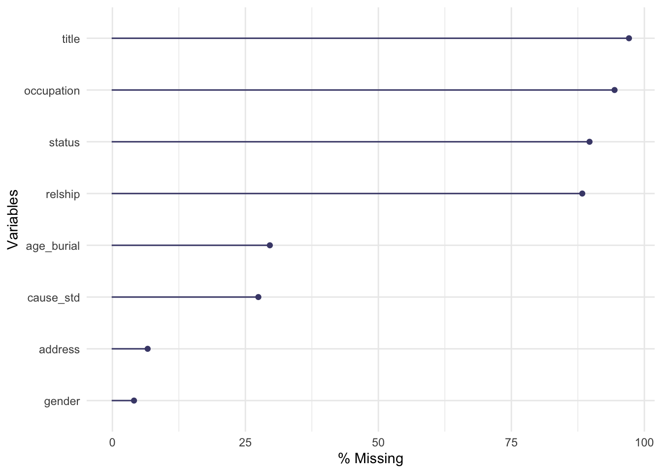
An overview
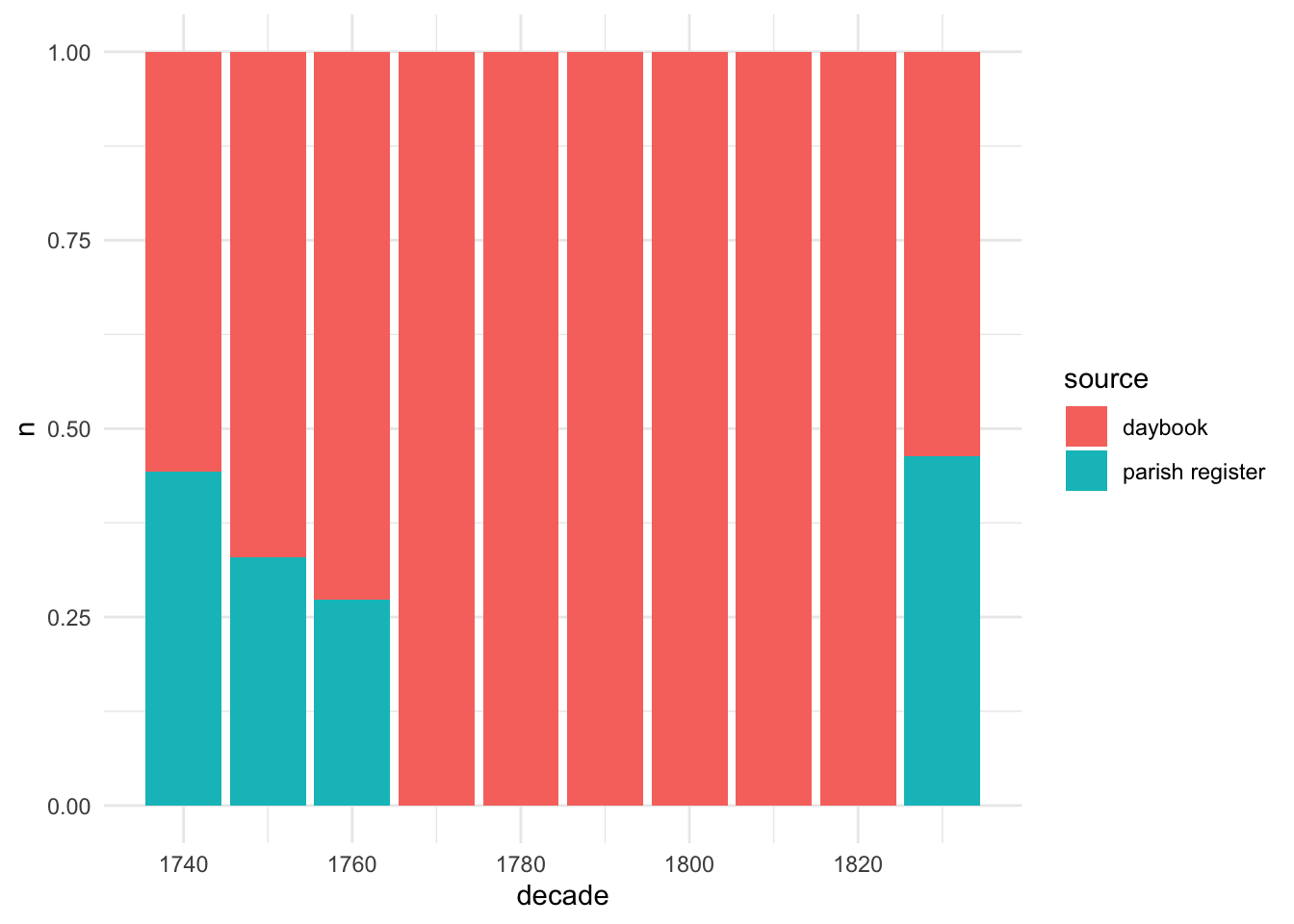
There are no missing dates; the original sources are chronological registers so the date was always recorded. (Which is often not the case for historical data!) The source (daybook or parish register) is also always present; this may be a significant variable when considering variations in missings.
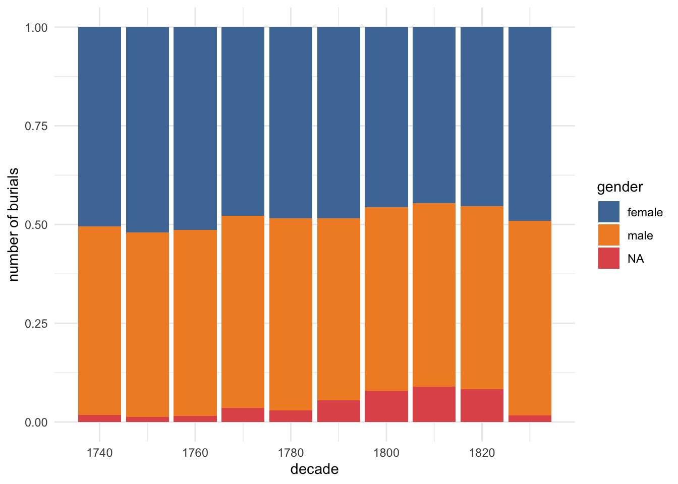
Gender needs to be considered separately, but my efforts seem to have been successful on first glance.
After that, there are massive variation in missingness.
address (which I think is generally parish level) is very well covered, with only 7% missing
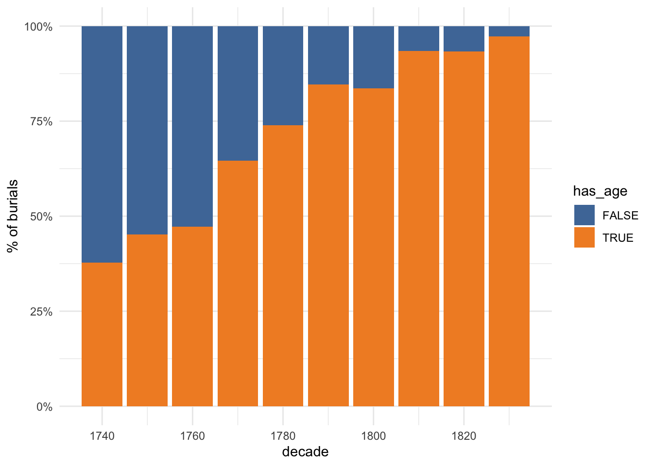
age and cause of death come next, around 30% missing
the other variables were only occasionally recorded
#warning seems to have gone with github version of naniar.#Warning: The `guide` argument in `scale_*()` cannot be `FALSE`. This was deprecated in ggplot2 3.3.4. Please use "none" instead.
More detailed analysis
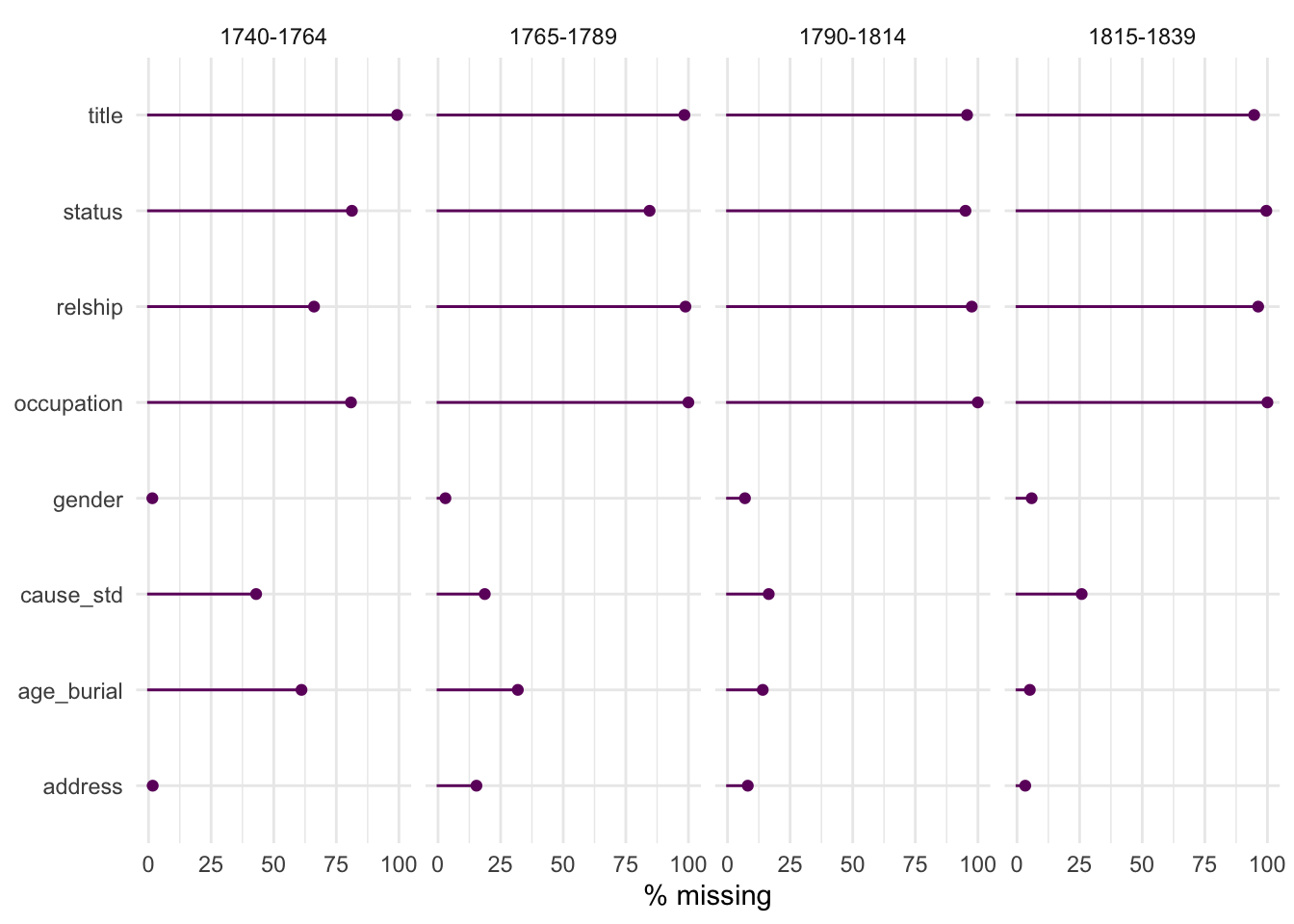
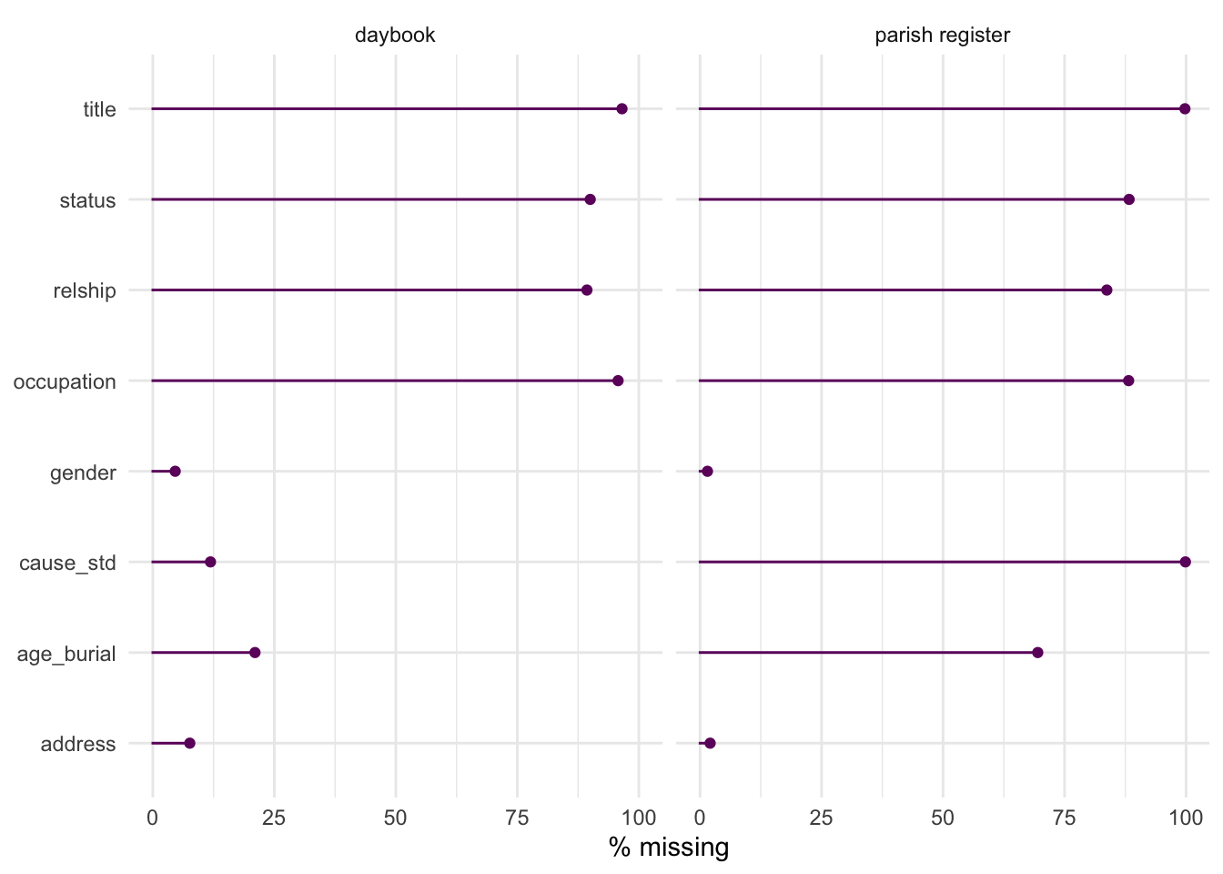
Since I know date is always present, I can use that to explore if or how much missing data might vary over time. I’ve split the dataset into four 25-year periods. I also want to know if there are significant differences between the two sources used.
Code
burials_1740_periods_missing_summary <-burials_1740 %>%select(status, occupation, gender, relship, age_burial, cause_std, address, period, title) %>%group_by(period) %>%miss_var_summary() %>%ungroup()burials_1740_source_missing_summary <-burials_1740 %>%select(status, occupation, gender, relship, age_burial, cause_std, address, source, title) %>%group_by(source) %>%miss_var_summary() %>%ungroup()#i think higher na gender in later decades is probably related to lack of status/relship data which you used to supplement names.burials_1740_periods_missing_summary %>%# select(status, occupation, gender, relship, age_burial, cause_std, address, period, title) %>%# group_by(period) %>%# miss_var_summary() %>%# ungroup() %>%ggplot(aes(variable, pct_miss)) +geom_col(width =0.001, colour ="#6e016b", fill ="#6e016b") +geom_point(colour ="#6e016b", fill ="#6e016b") +coord_flip() +facet_wrap(~period, nrow =1) +scale_color_discrete(guide ="none") +labs(y="% missing", x=NULL)
Code
# gg_miss_var(show_pct = TRUE, facet=county)
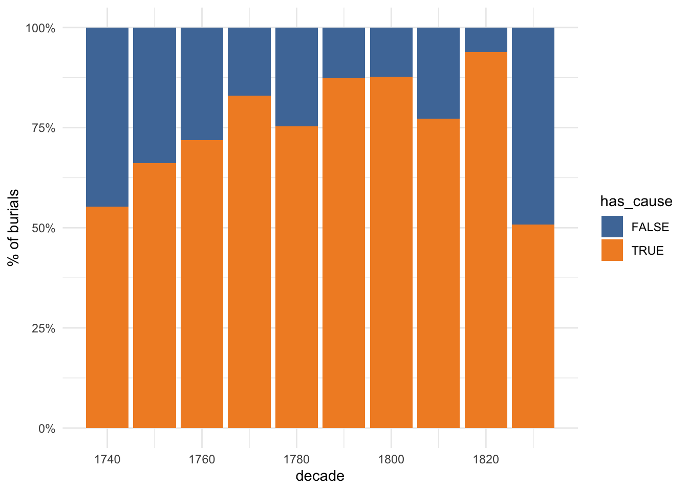
Now it’s possible to see that cause of death and age were recorded less often in the first decades of the dataset. In particular, in the 1740-64 period age was recorded only about 67% of the time but progressively improved until it was almost always recorded in 1815-39. Recording cause of death didn’t change quite as much, going from about 55% in 1740-64 to about 80% in 1790-1814 before getting slightly worse again in the last period.
With the gender data, significant variations might suggest, for example, that my data doesn’t reflect shifts in naming or spelling accurately. And it turns out there is some variation, from only 1.5% missing in 1740-64 but 7% in 1790-1814; although it’s all pretty good I’d want to work out why that’s happened and whether I can make it any better.
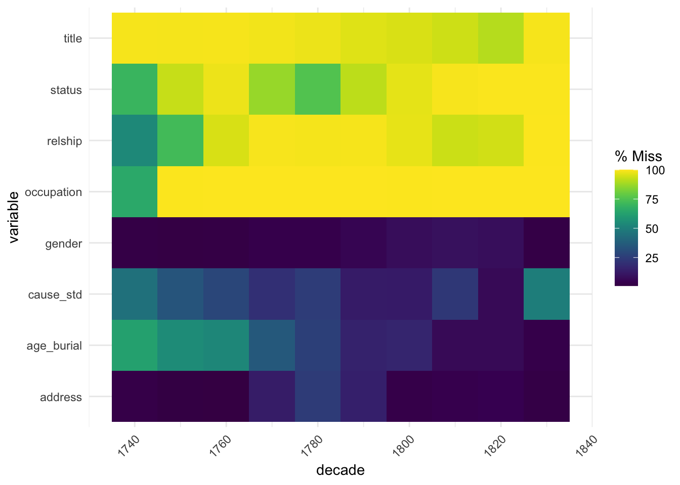
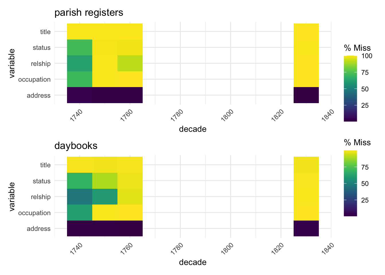
The naniar function gg_miss_fct creates a heatmap, and I think a breakdown by decade is particularly revealing. Lighter squares represent higher % missing within the decade, so (ignoring gender) we get a nice picture of shifts in recording information. Although as already noted, age and cause of death were less likely to be recorded in the early decades, occupation, status and relationship were all more likely to be recorded then than later on. Address was slightly less often recorded in the middle decades. There was also a noticeable decline in recording cause of death in the very last decade.
There are big differences in missing rates for the key data of cause of death and age between daybooks and parish registers. Cause of death is hardly ever recorded in parish registers (99.9% missing) and age is missing about 70% of the time, compared to 11.9% and 21% missing in daybooks.
(On the other hand, I’ve had a better success rate with gender in the parish registers - only 1.5% missing cf 4.6% in daybooks; maybe first names are recorded more often in registers.)
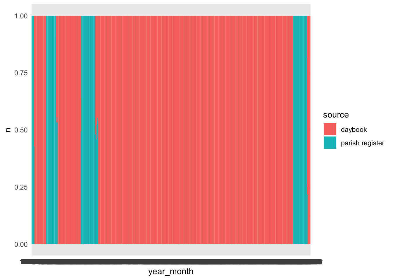
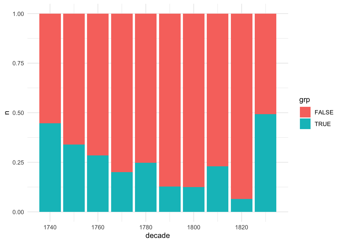
They’re not evenly spread; in fact, the dataset documentation makes it clear that daybooks were the main source and parish registers were used to fill in gaps - in other words, the dataset creators had a missing data problem, which they solved by using a different source.
Code
##parish register is clustered in two periods or 4 decades - 1740s-60s and 1830s (about half). [probably not enough dups to worry about which i preferred but presumably daybook since that's better on cause/age]burials_1740 %>%count(decade, source) %>%group_by(decade) %>%mutate(s=sum(n), p=n/s*100) %>%ungroup() %>%ggplot(aes(decade, n, fill=source)) +geom_col(position ="fill")
For some analysis (eg general changes over time, seasonal patterns), that won’t be a problem. It might not be a problem for the categories of cause of death and age that I’m interested in either, if the missing daybooks were MCAR (missing completely at random). Can I work out whether that’s the case?
To start with, it’s a promising sign that several other original variables - title, status, relship and occupation - have pretty similar missing data profiles overall and even when broken down by decade. This is the heatmap again for each source, showing only the decades in which parish registers have been used.
if you convert all parish register stuff (except dates!) to NA, what happens.
Code
burials_par <-burials_1740 %>%filter(decade %in%c(1740, 1750, 1760, 1830))#???? not sure if this will do anything usefulburials_par_na <-burials_1740 %>%mutate(across(c(title, forename, given, surname, gender, relship, relname, cause_std, address, occupation, status, age_group),~case_when( source=="parish register"~NA_character_,TRUE~ . ) )) %>%mutate(across(c(age_burial, age_group_n),~case_when( source=="parish register"~NA_real_,TRUE~ . ) ))
address? this is probably not very std though and recording habits might differ? but could do something like the top 20 huh, all the illegibles are in the daybook i think
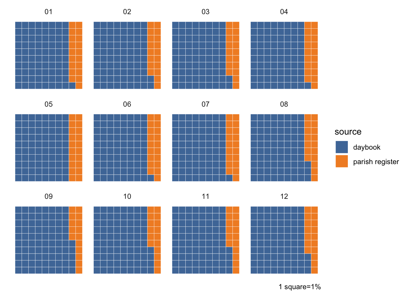
A potentially important factor is seasonality. It’s likely that there tend to be different causes of death at different times of year (and ages might vary seasonally too), so I hope that the daybook and parish register data have similar monthly patterns. Overall, parish registers make up 17.7% of the data, which varies by month between 15.5% (September) and 20.4% (May). In fact, lower % parish registers clearly cluster between the months of August and December.
Code
burials_1740 %>%count(month, source) %>%ggplot(aes(fill=source, values=n)) +geom_waffle(colour="white", n_rows =10, make_proportional =TRUE) +# can't remember how to fix ordering in waffle...coord_equal() +facet_wrap(~month) +theme_minimal() +theme_enhance_waffle() +scale_fill_tableau() +labs(fill="source", caption="1 square=1%")
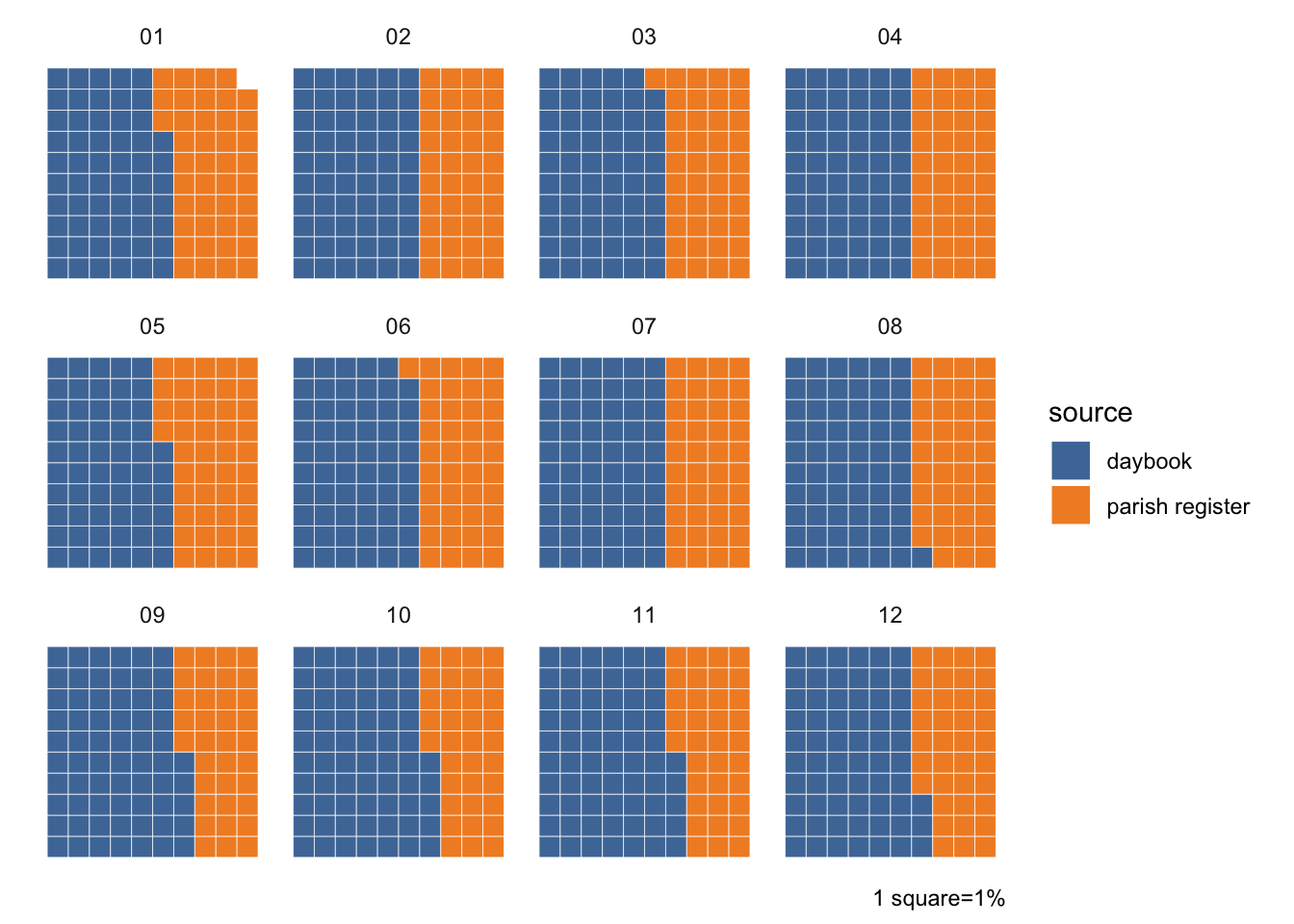
It might, however, be more appropriate to make the comparison only for decades in which parish registers have been used, rather than overall?
Code
burials_par %>%count(month, source) %>%ggplot(aes(fill=source, values=n)) +geom_waffle(colour="white", n_rows =10, make_proportional =TRUE) +# can't remember how to fix ordering in waffle...coord_equal() +facet_wrap(~month) +theme_minimal() +theme_enhance_waffle() +scale_fill_tableau() +labs(fill="source", caption="1 square=1%")
hmm, they’ve actually been filled in big chunks haven’t they, not interspersed.
then again some months have burials from both sources. those could be dups… there are quite a few dups in here ffs. they haven’t deduped because of age in a lot of cases. (a handful because of spelling variations in name)
Once we have a broad overview of missingness in the data, the next step is to explore how missingness exists at finer resolution within variables and cases. You might also refer to variables and cases as “columns” and “rows”, but for consistency, we will use “variables” and “cases”.
Gender
Code
sb_burials_na %>%count(decade, gender) %>%mutate(gender =replace_na(gender, "NA")) %>%ggplot(aes(decade, n, fill=gender)) +geom_col(position ="fill") +scale_fill_tableau() +labs(y="number of burials")
cause of death - 27.5% [25% all] have no cause of death
## NA cause# all data and 1740 are almost identical; does na cause skew towards early records?# slightly lower % f 46.5 (overall 47.8) - m 49.4 (48) but it's not far out.# burials_1740 %>%# filter(is.na(cause_std)) %>%# count(gender) %>%# mutate(p = n/sum(n)*100)
Code
## NA age# a bit more difference cf gender overall. f 45.4 and m 50.65# burials_1740 %>%# filter(is.na(age_burial)) %>%# count(gender) %>%# mutate(p = n/sum(n)*100)
# i appear to have some male died in childbirth... 6, and 12 NA...# 3 do have male names, but 3 have title "Mrs" - fixed. grrrrrr. but what other titles have you screwed up?# now 10 NA. (401 total childbirth)# burials_1740 %>%# filter(str_detect(cause_std, "childbirth")) %>%# filter(is.na(gender))# filter(gender=="male") # #filter(title=="Mrs") %>% count(gender)
Code
# some iffy ones here but I don't think there are any other systematic issues.# burials_1740 %>%# count(gender, title)
Code
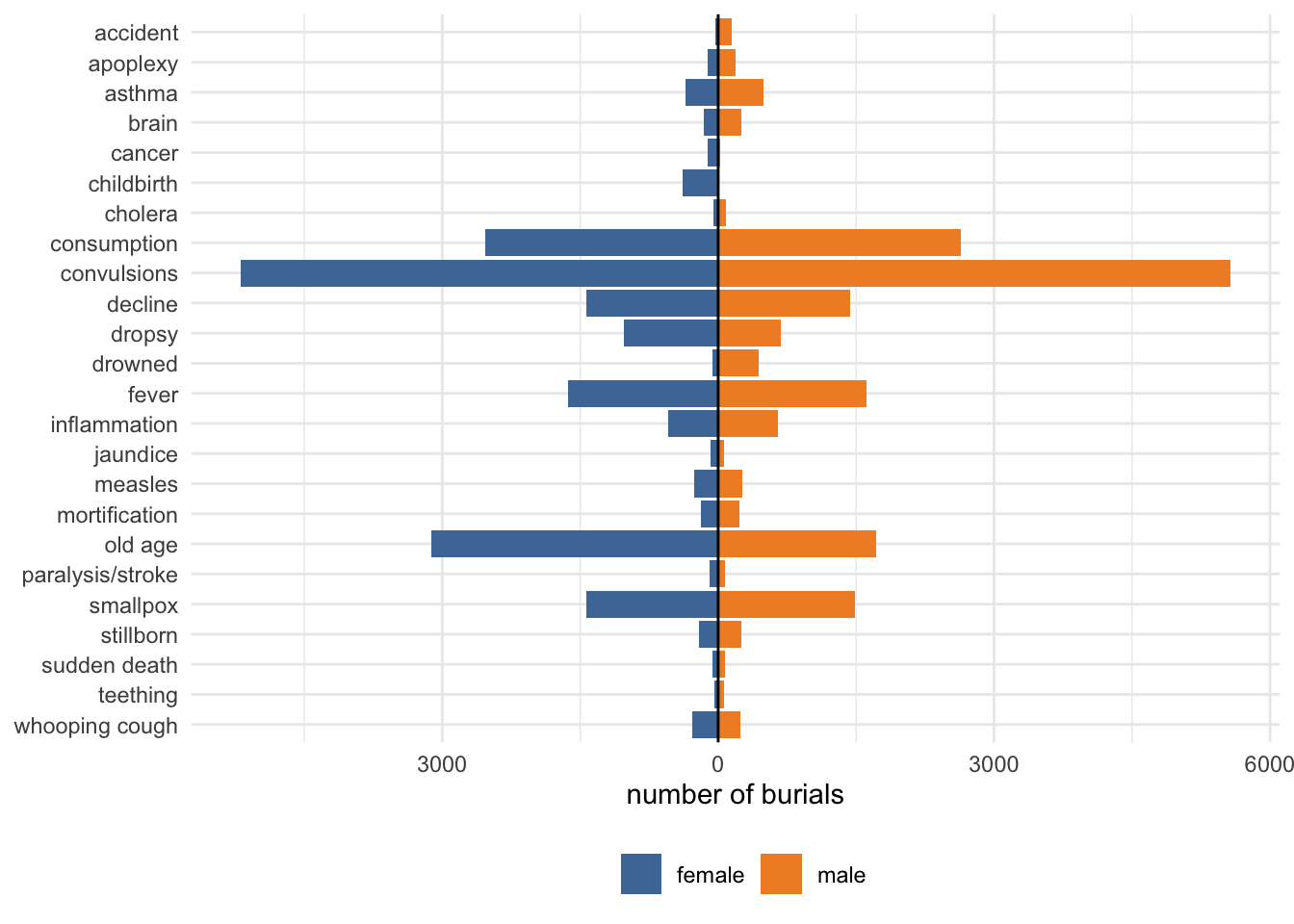
# diverging thingy is quite nice but hard to see smaller categoriesburials_1740_gender %>%filter(!is.na(cause_std)) %>%#mutate(cause_std = replace_na(cause_std, "n/a")) %>%add_count(gender, name="n_gen") %>%add_count(cause_std, name="n_cause") %>%filter(n_cause>100) %>%count(gender, n_gen, n_cause, cause_std, sort = T) %>%mutate(div_g =ifelse(gender=="female", n*-1, n)) %>%mutate(cause_std =fct_rev(cause_std)) %>%ggplot(aes(x=cause_std, fill=gender, y=div_g)) +geom_col() +coord_flip() +geom_hline(yintercept=0) +scale_y_continuous(labels=abs) +scale_fill_tableau() +theme(legend.position ="bottom") +labs(x=NULL, y="number of burials", fill=NULL)
Code
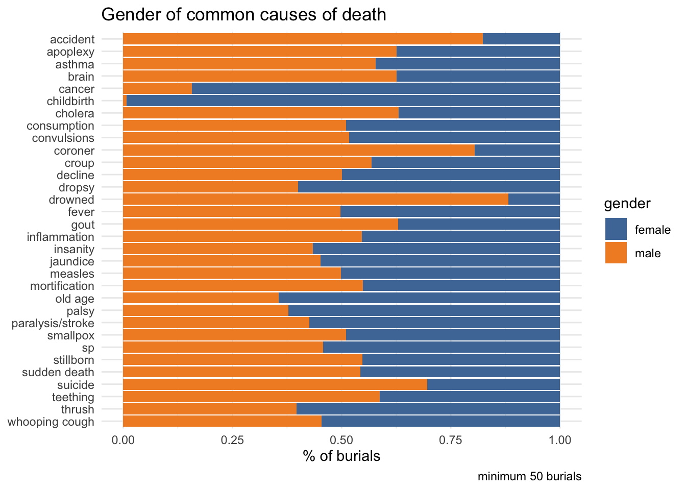
# wonder if this is a good one for a waffleburials_1740_gender %>%filter(!is.na(cause_std)) %>%#mutate(cause_std = replace_na(cause_std, "n/a")) %>%add_count(gender, name="n_gen") %>%add_count(cause_std, name="n_cause") %>%filter(n_cause>=50) %>%count(gender, n_gen, n_cause, cause_std, sort = T) %>%mutate(cause_std =fct_rev(cause_std)) %>%ggplot(aes(n, cause_std, fill=gender)) +geom_col(position ="fill") +scale_fill_tableau() +labs(y=NULL, x="% of burials", title ="Gender of common causes of death", caption ="minimum 50 burials")
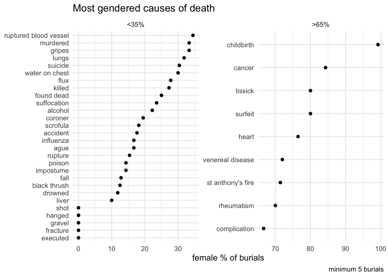
Most gendered causes of death
Code
burials_1740_gender %>%filter(!is.na(cause_std)) %>%#mutate(cause_std = replace_na(cause_std, "n/a")) %>%#add_count(gender, name="n_gen") %>%add_count(cause_std, name="n_cause") %>%filter(n_cause>4) %>%count(gender, n_cause, cause_std, sort = T) %>%pivot_wider(names_from = gender, values_from = n, values_fill =0) %>%mutate(female_p=round(female/n_cause*100, 2)) %>%filter(female_p>65| female_p<35) %>%mutate(fem_grp =if_else(female_p>65, ">65%", "<35%")) %>%mutate(cause_std =fct_reorder(cause_std, female_p)) %>%ggplot(aes(y=female_p, x=cause_std, group=fem_grp)) +geom_point() +#i've done lollipops with a line before. looks like it was geom_segment and kinda complicated... so ok.#ggalt::geom_lollipop(colour="lightgrey", point.colour = "black", horizontal=TRUE) + # this seems to force axis to start at 0 which is not helpful...coord_flip() +facet_wrap(~fem_grp, scales ="free") +labs(y="female % of burials", x=NULL, title ="Most gendered causes of death", caption ="minimum 5 burials")
Code
## stuff that isn't working...
Code
## Burial costs# no big difference here, which seems remarkable... well you can see some.# fees_1740 %>%# group_by(burial_id) %>%# summarise(fees_d = sum(fee_d)) %>%# ungroup() %>%# inner_join(burials_1740_gender, by="burial_id") %>%# filter(fees_d>0) %>% # there are 5 with 0 fees (=specified no fee) - causes a warning if using log scale# ggplot(aes(x=gender, y=fees_d, fill=gender)) +# lvplot::geom_lv(show.legend = F) +# #geom_boxplot() +# #ggbeeswarm::geom_beeswarm() +# #geom_violin() +# scale_y_log10() +# scale_fill_tableau() +# labs(y="total fees (d)", title = "Comparison of burial fees")
Code
# don't forget dplyr::summarise is masked by vcdExtra#library(vcd)#library(vcdExtra)
# ??don't really get this. but nb it can also be faceted.# sb_burials_na %>%# select(status, occupation, gender, relship, age_burial, cause_std, address) %>%# gg_miss_case(order_cases = F)
# don't think you have any facet options like ncol if you do it with gg_miss_var# burials_1740 %>%# mutate(p = case_when(# between(year, 1740, 1764) ~ "1740-1764",# between(year, 1765, 1789) ~ "1765-1789",# between(year, 1790, 1814) ~ "1790-1814",# between(year, 1815, 1839) ~ "1815-1839"# )) %>%# select(p, title, status, occupation, relship, age_burial, cause_std, address) %>%# gg_miss_var(facet = p)
Code
# Naniar has a function to create **upset plots**, which show how often missing variables *co-occur* (or correlate). They are cute but not necessarily easy to read and on this occasion I'm not sure it says anything very compelling, I think partly because missings tend to be either very high or low and not much in between. I've only selected some variables to make it easier to read.# burials_1740 %>%# select(age_burial, cause_std, address, occupation) %>%# gg_miss_upset()